Perlin Noise: A Procedural Generation Algorithm

This article is my humble attempt to explain how the algorithm works and how to use it.

It took me quite some time to understand how the algorithm works and a lot of resources helped me along the way. This is my way to return the favor.

Perlin noise is a popular procedural generation algorithm invented by Ken Perlin. It can be used to generate things like textures and terrain procedurally, meaning without them being manually made by an artist or designer. The algorithm can have 1 or more dimensions, which is basically the number of inputs it gets. In this article, I will use 2 dimensions because it’s easier to visualize than 3 dimensions. There is also a lot of confusion about what Perlin noise is and what it is not. It is often confused with value noise and simplex noise. There is basically 4 type of noise that are similar and that are often confused with one another : classic Perlin noise, improved Perlin noise, simplex noise, and value noise. Improved Perlin noise is an improved version of classic Perlin noise. Simplex noise is different but is also made by Ken Perlin. Value noise is also different. A rule of thumb is that if the noise algorithm uses a (pseudo-)random number generator, it’s probably value noise. This article is about improved Perlin noise.

First, how to use it. The algorithm takes as input a certain number of floating point parameters (depending on the dimension) and return a value in a certain range (for Perlin noise, that range is generally said to be between -1.0 and +1.0 but it’s actually a bit different). Let’s say it is in 2 dimensions, so it takes 2 parameters: x and y. Now, x and y can be anything but they are generally a position. To generate a texture, x and y would be the coordinates of the pixels in the texture (multiplied by a small number called the frequency but we will see that at the end). So for texture generation, we would loop through every pixel in the texture, calling the Perlin noise function for each one and decide, based on the return value, what color that pixel would be.

An example implementation would look like this:

Color pixels[500][500];

for (int y = 0; y < 500; y++) {
	for (int x = 0; x < 500; x++) {
		// Noise2D generally returns a value approximately in the range [-1.0, 1.0]
		float n = Noise2D(x*0.01, y*0.01);
		
		// Transform the range to [0.0, 1.0], supposing that the range of Noise2D is [-1.0, 1.0]
		n += 1.0;
		n /= 2.0;
		
		int c = Math.round(255*n);
		pixels[y][x] = Color(c, c, c);
	}
}

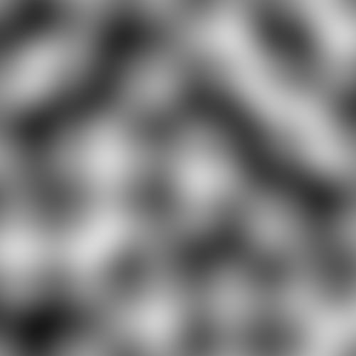
This code would result in an image like this:

[Figure 1]

The above code is in a C++-like language, where as all the rest of the code is in ES6 javascript.

Also, the code has been written for readability, not performance. It creates a lot of unnecessary temporary Vector2 objects. If you want to use Perlin noise for a real-world project, I recommend using a more standard (and faster) implementation, like Ken Perlin’s reference implementation. You could even use some noise functions that are implemented entirely on the GPU, which is generally much faster than a CPU implementation.

As you can see, each pixel don’t just have a random color, instead they follow a smooth transition from pixel to pixel and the texture don’t look random at the end. That is because Perlin noise (and other kinds of noise) has this property that if 2 inputs are near each other (e.g. (3.1, 2.5) and (3.11, 2.51)), the results of the noise function will be near each other too.

So, how does it work?

I’ll give a quick explanation first and explain it in details later:

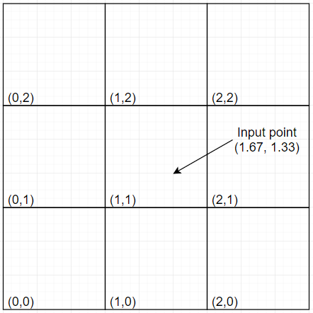
The inputs are considered to be on an integer grid (see Figure 2). Each floating point input lies within a square of this grid. For each of the 4 corners of that square, we generate a value. Then we interpolate between those 4 values and we have a final result. The difference between Perlin noise and value noise is how those 4 values are obtained. Where value noise uses a pseudo-random number generator, Perlin noise does a dot product between 2 vectors.

[Figure 2]

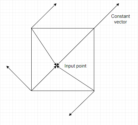
The first vector is the one pointing from the grid point (the corners) to the input point. The other vector is a constant vector assigned to each grid point (see Figure 3). That one must always be the same for the same grid point, but it can change if you change the seed of the algorithm (we’ll see how in a moment).

[Figure 3]

An implementation to get the first vector would look like this:

// Suppose x, y and z are the float input
const X = Math.floor(x) & 255;	// Used later
const Y = Math.floor(y) & 255;	// Used later
const xf = x-Math.floor(x);
const yf = y-Math.floor(y);

const topRight = new Vector2(xf-1.0, yf-1.0);
const topLeft = new Vector2(xf, yf-1.0);
const bottomRight = new Vector2(xf-1.0, yf);
const bottomLeft = new Vector2(xf, yf);

Generally, in Perlin noise implementations, the noise will “wrap” after every multiple of 256 (let’s call this number w), meaning it will repeat. That’s because, to give every grid point a constant vector, we’ll soon need something called a permutation table. It’s an array of size w containing all the integers between 0 and w-1 but shuffled (i.e. a permutation). The index for this array (the value between the square brackets [ ]) is X or Y (or a value near them) so it need to be less than 256. The noise “wraps” because if, for example, the input x is 256, X will be equal to 0. This 0 will be used to index the permutation table and then to generate a random vector. Since X is 0 at every multiple of 256, the random vector will be the same at all those points, so the noise repeats. You can if you want have a larger permutation table (say, of size 512) and in that case the noise would wrap at every multiple of 512.

The thing is, that’s just the technique used by Ken Perlin to get those constant vectors for each corner point. You can absolutely use another way, and you would maybe not have the limitation of the wrapping. You could for example use a pseudo random number generator to generate the constant vectors, but in this case you would probably fair better by just using value noise.

We first create the permutation table and shuffle it. I’ll show you the code and I’ll explain just after:

// Create an array (our permutation table) with the values 0 to 255 in order
const permutation = [];
for(let i = 0; i < 256; i++) {
	permutation[i] = i;
}

// Shuffle it
permutation = Shuffle(permutation);

An example of a shuffle function is given in the complete code at the end of the article.

Next, we need a value from that table for each of the corners. There is a restriction however: a corner must always get the same value, no matter which of the 4 grid cells that has it as a corner contains the input value. For example, if the top-right corner of the grid cell (0, 0) has a value of 42, then the top-left corner of grid cell (1, 0) must also have the same value of 42. It’s the same grid point, so same value no matter from which grid cell it’s calculated:

// Select a value in the array for each of the 4 corners
const valueTopRight = P[P[X+1]+Y+1];
const valueTopLeft = P[P[X]+Y+1];
const valueBottomRight = P[P[X+1]+Y];
const valueBottomLeft = P[P[X]+Y];

The way we selected the values for the corners in the code above respect this restriction. If we are in grid cell (0, 0), “valueBottomRight” will be equal to P[P[0+1]+0] = P[P[1]+0]. Whereas in the grid cell (1, 0), “valueBottomLeft” will be equal to P[P[1]+0]. “valueBottomRight” and “valueBottomLeft” are the same. The restriction is respected.

We also want to double the table for the noise to wrap at each multiple of 256. If we are computing P[X+1] and X is 255 (so X+1 is 256), we would get an overflow if we didn’t double the array because the max index of a size 256 array is 255. What is important is that we must not double the array and then shuffle it. Instead, we must shuffle it and then double it. In the example of P[X+1] where X is 255, we want P[X+1] to have the same value as P[0] so the noise can wrap.

Now is the time to get those constant vectors. Ken Perlin’s original implementation used a strange function called “grad” that calculated the dot product for each corner directly. We are gonna make things simpler by creating a function that just returns the constant vector given a certain value from the permutation table and calculate the dot product later.

Also, since it’s easier to generate them, those constant vectors can be 1 of 4 different vectors: (1.0, 1.0), (1.0, -1.0), (-1.0, -1.0) and (-1.0, 1.0).

To find the constant vectors given a value from a permutation table, we can do something like that:

function GetConstantVector(v) {
	// v is the value from the permutation table
	const h = v & 3;
	if(h === 0)
		return new Vector2(1.0, 1.0);
	else if(h === 1)
		return new Vector2(-1.0, 1.0);
	else if(h === 2)
		return new Vector2(-1.0, -1.0);
	else
		return new Vector2(1.0, -1.0);
}

Since v is between 0 and 255 and we have 4 possible vectors, we can do a & 3 (equivalent to % 4) to get 4 possible values of h (0, 1, 2 and 3). Depending of that value, we return one of the possible vectors.

We can now calculate the dot products:

const dotTopRight = topRight.dot(GetConstantVector(valueTopRight));
const dotTopLeft = topLeft.dot(GetConstantVector(valueTopLeft));
const dotBottomRight = bottomRight.dot(GetConstantVector(valueBottomRight));
const dotBottomLeft = bottomLeft.dot(GetConstantVector(valueBottomLeft));

Now that we have to dot product for each corner, we need to somehow mix them to get a single value. For this, we’ll use interpolation. Interpolation is a way to find what value lies between 2 other values (say, a1 and a2), given some other value t between 0.0 and 1.0 (a percentage basically, where 0.0 is 0% and 1.0 is 100%). For example: if a1 is 10, a2 is 20 and t is 0.5 (so 50%), the interpolated value would be 15 because it’s midway between 10 and 20 (50% or 0.5). Another example: a1=50, a2=100 and t=0.4. Then the interpolated value would be at 40% of the way between 50 and 100, that is 70. This is called linear interpolation because the interpolated values are in a linear curve.

Now we have 4 values that we need to interpolate but we can only interpolate 2 values at a time. So to way we use interpolation for Perlin noise is that we interpolate the values of top-left and bottom-left together to get a value we’ll call v1. After that we do the same for top-right and bottom-right to get v2. Then finally we interpolate between v1 and v2 to get a final value. This is the value we want our noise function to return.

Note that if we change the input point just a little bit, the vectors between each corner and the input point will change just a little bit too, whereas the constant vector will not change at all. The dot products will also change just a little bit, and so will the final value return by the noise function. Even if the input changes grid square, like from (3.01, 2.01) to (2.99, 1.99), the final values will still be very close because even if 2 (or 3) of the corners change, the other 2 (or 1) would not and since with both inputs we are close to the corner(s), interpolation will cause the final value to be really close to that of the corner(s). Since with both inputs that corner will have the same value, the final results will be really close.

Here is the code for a function that does linear interpolation (also called lerp):

function Lerp(t, a1, a2) {
	return a1 + t*(a2-a1);
}

We could use linear interpolation but that would not give great results because it would feel unnatural, like in this image that shows 1 dimensional linear interpolation :

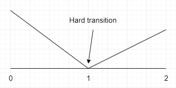
[Figure 4] The abrupt transition that results from linear interpolation

As you can see, the change between what is inferior to 1 and what is superior to 1 is abrupt. What we want is something smoother, like this:

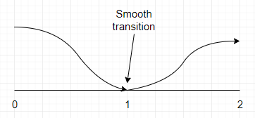
[Figure 5] The smooth transition that results from non-linear interpolation

Or in 2D:

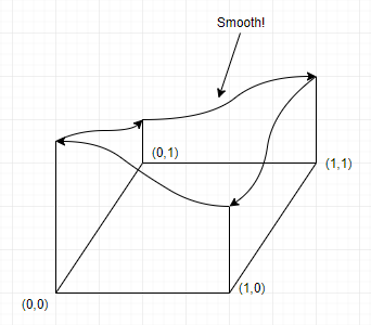
[Figure 6] The smooth transition between the corners of a grid square

With linear interpolation, we would use xf as an interpolation value (t). Instead we are going to transform xf and yf into u and v. We will do it in a way that, given a value of t between 0.0 and 0.5 (excluded), the transformed value will be something a little bit smaller (but capped at 0.0). Also, given a value of t between 0.5 (excluded) and 1.0, the transformed value would be a little larger (but capped at 1.0). For 0.5, the transformed value should be 0.5. Doing this will result in a curvy transition, like in figures 5 and 6.

To do this, we need something called an ease curve: it’s just a mathematical curve that looks like this:

[Figure 7] An ease curve

If you look closely, you can see that for an input (xf or yf, the x axis) between 0.0 and 0.5, the output (u or v, the y axis) is a little bit closer to 0.0. And for a value between 0.5 and 1.0, the output is a little bit closer to 1.0. For x=0.5, y=0.5. That will do the work perfectly.

The curve above is the ease function used by Ken Perlin in his implementation of Perlin Noise. The equation is 6t5-15t4+10t3. This is also called a fade function. In code, it looks like that:

// Unoptimized version
function Fade(t) {
	return 6*t*t*t*t*t - 15*t*t*t*t + 10*t*t*t;
}

// Optimized version (less multiplications)
function Fade(t) {
	return ((6*t - 15)*t + 10)*t*t*t;
}

Now, we just have to do linear interpolation the way we said before, but with u and v as interpolation values (t). Here is the code:

const u = Fade(xf);
const v = Fade(yf);
const result = Lerp(u,
	Lerp(v, dotBottomLeft, dotTopLeft),
	Lerp(v, dotBottomRight, dotTopRight)
);

That’s it! Perlin noise completed. Here’s the full code:

class Vector2 {
	constructor(x, y) {
		this.x = x;
		this.y = y;
	}

	dot(other) {
		return this.x*other.x + this.y*other.y;
	}
}

function Shuffle(arrayToShuffle) {
	for(let e = arrayToShuffle.length-1; e > 0; e--) {
		const index = Math.round(Math.random()*(e-1));
		const temp = arrayToShuffle[e];
		
		arrayToShuffle[e] = arrayToShuffle[index];
		arrayToShuffle[index] = temp;
	}
}

function MakePermutation() {
	const permutation = [];
	for(let i = 0; i < 256; i++) {
		permutation.push(i);
	}

	Shuffle(permutation);
	
	for(let i = 0; i < 256; i++) {
		permutation.push(permutation[i]);
	}
	
	return permutation;
}
const Permutation = MakePermutation();

function GetConstantVector(v) {
	// v is the value from the permutation table
	const h = v & 3;
	if(h == 0)
		return new Vector2(1.0, 1.0);
	else if(h == 1)
		return new Vector2(-1.0, 1.0);
	else if(h == 2)
		return new Vector2(-1.0, -1.0);
	else
		return new Vector2(1.0, -1.0);
}

function Fade(t) {
	return ((6*t - 15)*t + 10)*t*t*t;
}

function Lerp(t, a1, a2) {
	return a1 + t*(a2-a1);
}

function Noise2D(x, y) {
	const X = Math.floor(x) & 255;
	const Y = Math.floor(y) & 255;

	const xf = x-Math.floor(x);
	const yf = y-Math.floor(y);

	const topRight = new Vector2(xf-1.0, yf-1.0);
	const topLeft = new Vector2(xf, yf-1.0);
	const bottomRight = new Vector2(xf-1.0, yf);
	const bottomLeft = new Vector2(xf, yf);
	
	// Select a value from the permutation array for each of the 4 corners
	const valueTopRight = Permutation[Permutation[X+1]+Y+1];
	const valueTopLeft = Permutation[Permutation[X]+Y+1];
	const valueBottomRight = Permutation[Permutation[X+1]+Y];
	const valueBottomLeft = Permutation[Permutation[X]+Y];
	
	const dotTopRight = topRight.dot(GetConstantVector(valueTopRight));
	const dotTopLeft = topLeft.dot(GetConstantVector(valueTopLeft));
	const dotBottomRight = bottomRight.dot(GetConstantVector(valueBottomRight));
	const dotBottomLeft = bottomLeft.dot(GetConstantVector(valueBottomLeft));
	
	const u = Fade(xf);
	const v = Fade(yf);
	
	return Lerp(u,
		Lerp(v, dotBottomLeft, dotTopLeft),
		Lerp(v, dotBottomRight, dotTopRight)
	);
}

If you run the code and try to generate something like a texture, giving to the Noise function the coordinates of it’s pixels, you will probably get a completely black texture.

Why?

When all the input to the algorithm are integers, say (5,3), the vector from the grid point (5,3) to the input will be the vector (0,0), because the input is also (5,3). The dot product for that grid point will be 0, and since the input lies exactly on that grid point, the interpolation will cause the result to be exactly that dot product, that is, 0. To solve this small issue, we generally multiply the inputs by a small value called the frequency.

Here is an example of Perlin noise for generating a heightmap.

Fractal brownian motion (FBM)

Fractal brownian motion is not part of the core Perlin noise algorithm, but it is (as far as I know) almost always used with it. It gives MUCH better results:

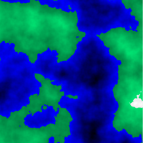
[Figure 8] A colored heightmap generated with Perlin noise with fractal brownian motion

Now without FBM:

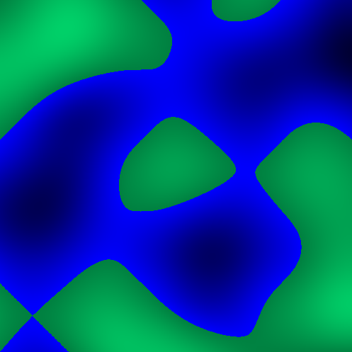
[Figure 9] A colored “heightmap” generated with Perlin noise without fractal brownian motion

So how does it work?

The second image doesn’t look good because it is way too smooth, which make it unrealistic. Real life terrain is more noisy.

So to go from the second image to the first, we need to add some noise, and luckily for us, this is basically what FBM does.

Here is what 1 dimensional Perlin noise might look like with the input x being a real number between 0 and 3, and with a frequency of 1 :

[Figure 10] 1 dimensional Perlin noise with frequency of 1

If we take another curve with an input x between 0 and 3 but use a frequency of 2, it will look like this :

[Figure 11] 1 dimensional Perlin noise with frequency of 2

Even though the input is still between 0 and 3, the curve look a lot bumpier because multiplying the input by 2 made it effectively go from 0 to 6. What if we multiplied this curve by some value between 0 and 1 (let’s say 0.5) and added it to the first curve?

We would get this :

[Figure 12] 2 octaves of Perlin noise

If we add another of these curves, also doubling the frequency and decreasing the multiplier (which is called the amplitude), we would get something like this :

[Figure 13] 3 octaves of Perlin noise

If we keep doing this a few more times, we would get this :

[Figure 14] 8 octaves of Perlin noise

This is exactly what we want. A curve with an overall smooth shape, but with a lot of smaller details. This look like a realistic chain of moutains. If you do this in 2d, it’s exactly how you get the heightmap from Figure 8.

We just added multiple “layers” of noise together, each with a different amplitude and frequency, and when one layer has a frequency that is double the frequency of the previous layer, this layer is called an octave. Though you will probably often see the term “octave” used more loosely for when the frequency is multiplied by a number other than 2.

The first octave constitute the overall shape of our chain of mountains. It has a small frequency (so there is not a million moutains) and an amplitude of 1. The second octave will add smaller (so we decrease the amplitude) more noisy details to the mountain range (so we increase the frequency). We can keep doing this - adding smaller and smaller details to the moutains - until we have our final (and beautiful) result.

You don’t have to worry about the final value exceeding the typical range of Perlin noise because even though we keep adding stuff, those stuff are not all positive, they can also be negative, so it balances out. Also, we keep decreasing the amplitude so we are adding smaller and smaller numbers, which diminishes the chances of overflowing the range. But still, it will happen sometimes.

In code, it would look something like this:

function FractalBrownianMotion(x, y, numOctaves) {
	let result = 0.0;
	let amplitude = 1.0;
	let frequency = 0.005;

	for (let octave = 0; octave < numOctaves; octave++) {
		const n = amplitude * Noise2D(x * frequency, y * frequency);
		result += n;
		
		amplitude *= 0.5;
		frequency *= 2.0;
	}

	return result;
}

There you go. This is Perlin noise in a nutshell. You can use it to generate all kinds of things, from moutains ranges to heightmaps.

Hope you liked. Thanks for reading :)